One of the most annoying parts of writing publishable research material is making figures. Although it may seem rather simple to make a figures from, say, a spreadsheet program, systematic generation of high-quality figures is not that easy. I decided to write this post as a guide to my fellow lab members, and thought it may be useful to other researchers as well. The system described here is mainly based on the excellent matlab2tikz package.

How hard is it to make a nice figure out of Matlab?

I am going to argue that the answer is very hard. Now of course anyone having used Matlab knows of the plot and saveas functions, and is able to quickly produce a figure using something like this:

x = [0:0.01:1];
y = x+0.1.*randn(1,length(x));
h=figure;
plot(x,y)
xlabel('X [m]')
ylabel('Y [s]')
saveas(h,'fig1.jpg')

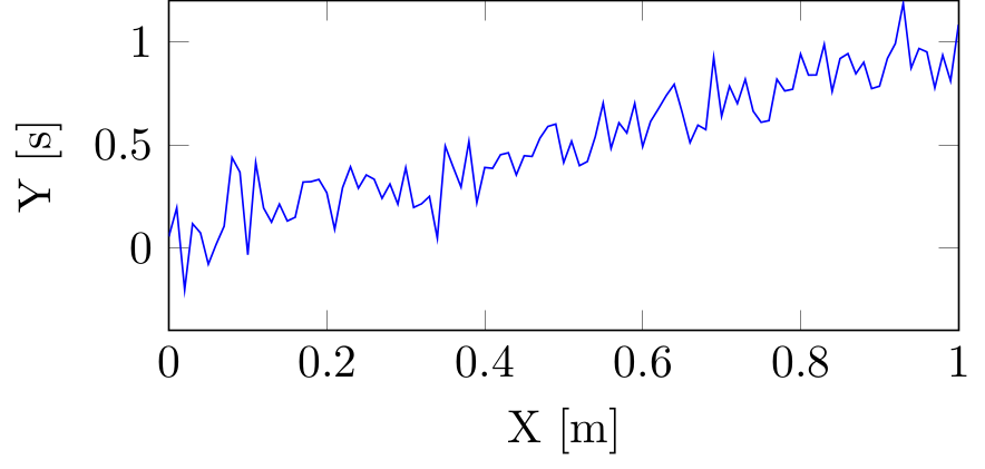
Which results in the following image.

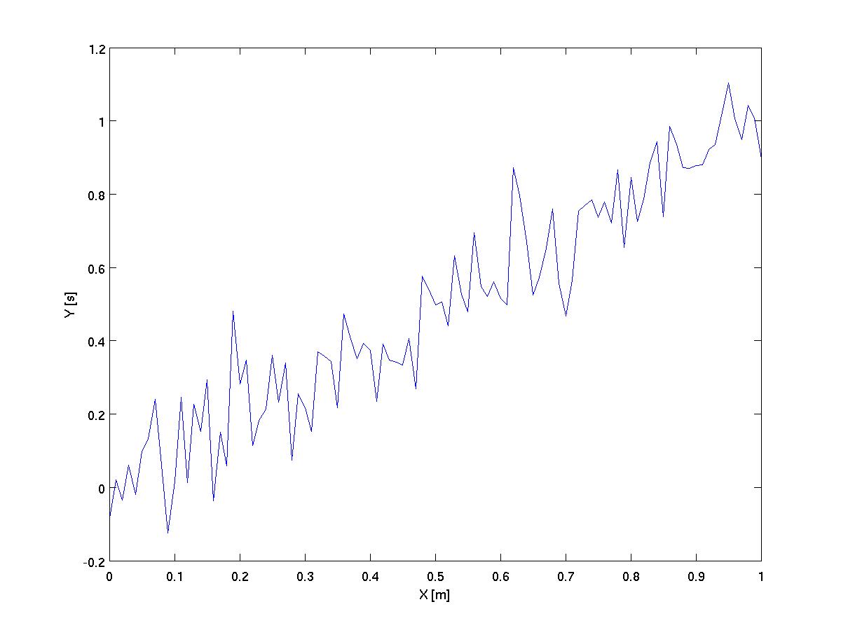
This figure is certainly fine, but the fonts are too small, not to mention ugly, and the line is too thin. This can of course be remedied by using the export setup feature before saving the figure. Loading the default presentation parameters, for instance, and saving as before, gives us the following image.

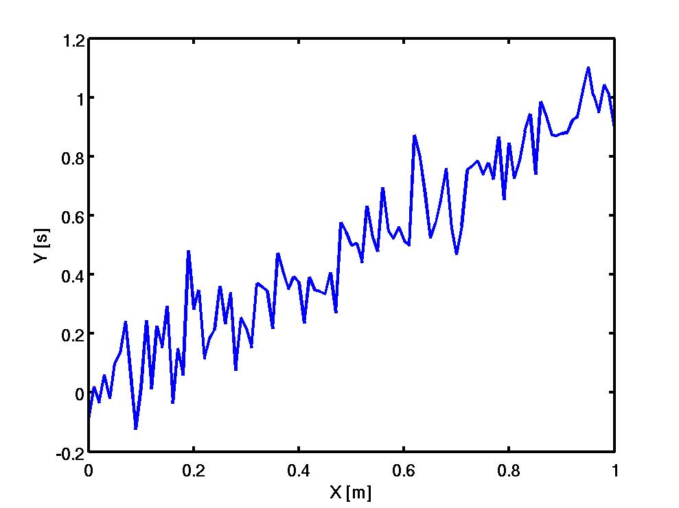
This is better. The fonts look better, and the line is thick enough to be easily seen. This figure could almost be put in a poster. But as always, the devil is in the details. The first problem we notice is the jpg compression. On a poster, this will be really noticeable. So let’s use a loss-less format, like png.

Now this we could put in a poster… maybe. We may still need to change the font to something like Helvetica to be in accordance with the rest of the text. But for the most part, this is probably fine. If we want to be really picky, we can always remove all text from this figure.

set(gca,'YTickLabel',[])
set(gca,'XTickLabel',[])

This way we can insert all the text (tick labels, axis labels, etc.) directly in whatever program we use for making the poster. I made many of my posters in this way, except that I used vector graphics.

Vector graphics

So far, we used raster formats to save our figure. In raster formats (bitmap, jpeg, png, gif, tiff etc.), the colour of each pixel in the image is independently stored. A bitmap image, for instance, is simply an array of colours, each for one pixel of the image. Vector graphics, on the other hand, store data about how the image was generated. For example, a vector image file can simple contain a line telling the viewer to draw a circle, instead of defining the value of all pixels in the image.

The great advantage of vector formats over raster formats is the the former can be arbitrarily resized without any loss in quality. If our figure was smaller, resizing it to be larger would cause it to look like this:

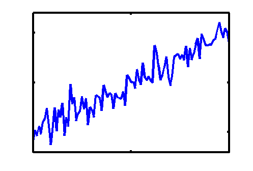
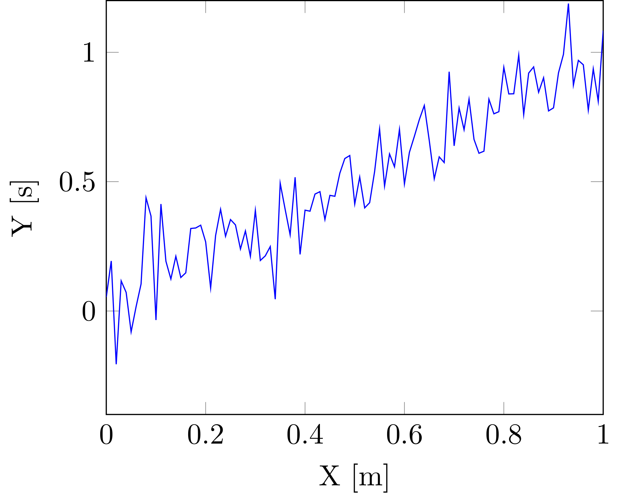
Those jagged line (steps) are due to the resizing of the image. We can avoid them by storing our figure in a vectorial format, such as svg. Matlab can not do this out of the box, but we can use an external script for this. One such script can be found here. The same figure saved as an svg image looks like this:

So here we have it. Make Matlab figures. Set the right options (remove all text, change line width, etc.). Save them as vector graphics (eps is fine, and included in matlab). Add text accordingly. If you are using Windows, you can also copy and paste Matlab figures directly into powerpoint or word. This works for the most part pretty well and you can also safely resize the resulting figure directly in powerpoint. I don’t use windows, so I usually used the eps format.

There are other problems associated with this approach. There is a lot of manual work involved, which makes the process very error-prone. In addition, adding the text externally is really only feasible for a poster. If you are writing a document, either in a word processor or using LaTeX, this becomes impractical. Another problem with this approach is visible in the last figure. Resizing the figure also resized the lines, points, and any text in the figure. In the last figure, the line is way too thick. This means that the figures need to be created at the right size inside Matlab, before being exported. This means that figures can not be made once, and used for different posters/papers/etc.

These problems led me to use tikz for figures in my thesis. In the rest of this post, I will explain the basics of using tikz to create a figure and including tikz figures inside LaTeX documents.

Making figures with tikz

Here is the basic code to generate and export our figure to tikz.

set(0,'defaulttextinterpreter','none'); % Prevents Matlab from trying to
    % interpret latex string.
h=figure;
plot(x,y);
xlabel('X [m]');
ylabel('Y [s]');
cleanfigure;
matlab2tikz('fig6.tikz', 'showInfo', false, ...
        'parseStrings',false,'standalone', true, ...
        'height', '5cm', 'width','6cm');

Running this chuck of code will give us a tikz file. A tikz file basically contains instructions that can be understood by a latex interpreter to produce an image. In this case, the tikz file uses another package, pgfplot, which provides commands to easily draw axes and coordinates. Our tikz file contains :

% This file was created by matlab2tikz v0.4.4 running on MATLAB 8.2.
% Copyright (c) 2008--2013, Nico Schlömer <nico.schloemer@gmail.com>
% All rights reserved.
%
\documentclass[tikz]{standalone}
\usepackage{pgfplots}
\pgfplotsset{compat=newest}
\usetikzlibrary{plotmarks}
\usepackage{amsmath}

\begin{document}
\begin{tikzpicture}

\begin{axis}[%
width=6cm,
height=5cm,
scale only axis,
xmin=0,
xmax=1,
xlabel={X [m]},
ymin=-0.4,
ymax=1.2,
ylabel={Y [s]}
]
\addplot [
color=blue,
solid,
forget plot
]
table[row sep=crcr]{
0 0.05376671395461\\
0.01 0.193388501459509\\
0.02 -0.205884686100365\\
0.03 0.116217332036812\\
0.04 0.0718765239858981\\
0.05 -0.0807688296305274\\
0.06 0.0166407977694316\\
0.07 0.104262446653865\\
0.08 0.437839693972576\\
0.09 0.366943702988488\\
...
0.99 0.810532115854488\\
1 1.08403755297539\\
};
\end{axis}
\end{tikzpicture}%
\end{document}

This is actually human readable. You could, if you wanted to, dig in and change anything about the figure. Since it is a plain-text file, you could also automate these changes. Imagine that instead of putting voltage on one of your axes, you wanted to use potential. You could do that for all the figures in one folder by running a command like:

sed 's/voltage/potential/g' *.tikz

We can also use all sorts of tools that work nicely with plain-text files, such as version control systems. The tikz file can be converted into a pdf file by running on the command line (not in matlab):

lualatex fig6.tikz

This creates a pdf file, that looks like this:

Crucially, changing the width and height on the tikz file, and regenerating the pdf file results in a figure that looks as good. If we divide the height by 2, we get the following figure:

The width of the line, the shape and the placement of text labels are all preserved perfectly, and of course, the pdf being a vectorial format, there is no jaggedness or steps.

Inside a LaTeX document

The advantages of this workflow, even though the generated figures are gorgeous, are not obvious so far. Instead of having a tikz file, we could also have saved the matlab figure as .fig file and exported from it as a .tiff file in the right size anytime we needed to. With the tikz format, we have to modify the .tikz file and recompile it every time we need a different sized figure. This can be done programmatically thanks to the plain-text format, but is far from being really practical.

Where this method really shows its potential is inside a LaTeX document. Instead of compiling the figure into a pdf file to be included in the pdf generated by LaTeX, you can import the tikz file directly. First, we need to generate a non-standalone tikz file. This can be done by running the matlab2tikz command with the standalone option set to false:

matlab2tikz('fig8.tikz', 'showInfo', false, ...
        'parseStrings',false,'standalone', false, ...
        'height', '\figureheight', 'width','\figurewidth');

Notice that instead of specifying a width and a height, we give two LaTeX comamnds: \figurewidth and \figureheight. These are not standard latex commands. We will define them in our LaTeX document. The generated tikz file contains:

% This file was created by matlab2tikz v0.4.4 running on MATLAB 8.2.
% Copyright (c) 2008--2013, Nico Schlömer <nico.schloemer@gmail.com>
% All rights reserved.
%
\begin{tikzpicture}

\begin{axis}[%
width=\figurewidth,
height=\figureheight,
scale only axis,
xmin=0,
xmax=1,
xlabel={X [m]},
ymin=-0.4,
ymax=1.2,
ylabel={Y [s]}
]
\addplot [
color=blue,
solid,
forget plot
]
table[row sep=crcr]{
0 0.05376671395461\\
0.01 0.193388501459509\\
0.02 -0.205884686100365\\
...
0.99 0.810532115854488\\
1 1.08403755297539\\
};
\end{axis}
\end{tikzpicture}%

We cannot directly compile this file into a pdf document. Instead, this file can be included inside a LaTeX document:

\documentclass[a4paper]{article}
\usepackage[utf8]{inputenc}
\usepackage[english]{babel}
\usepackage{tikz, pgfplots} % Necessary package for tikz
\usepackage[font=normal,labelfont=bf]{caption}
\pgfplotsset{ % Here we specify options for all figures in the document
  compat=1.8, % Which version of pgfplots do we want to use?
  legend style = {font=\small\sffamily}, % Legends in a sans-serif font
  label style = {font=\small\sffamily} % Labels in a sans-serif font
}
\begin{document}
\newlength\figureheight
\newlength\figurewidth

\begin{figure}[h]
  \setlength\figureheight{0.3\textwidth}
  \setlength\figurewidth{0.8\textwidth}
  \input{fig8.tikz}%
  \caption{\label{fig:1}Our figure}
\end{figure}

\begin{figure}[h]
  \setlength\figureheight{0.6\textwidth}
  \setlength\figurewidth{0.8\textwidth}
  \input{fig8.tikz}%
  \caption{\label{fig:2}Our figure, with a different size}
\end{figure}

\end{document}

There are a few remarkable things about this document. First of all, notice that we define parameter for the figure inside the LaTeX document. For instance, we decide to use a sans-serif font for all the figures in the document, as opposed to the one used in the standalone case. We also define two latex variables, \figrelength and \figureheight, using the \newlength command. We can change the values of these variable before we include each figure (using \input). This is how we can create figures with different heights from the same original tikz file. Compiling this LaTeX document creates this pdf file:

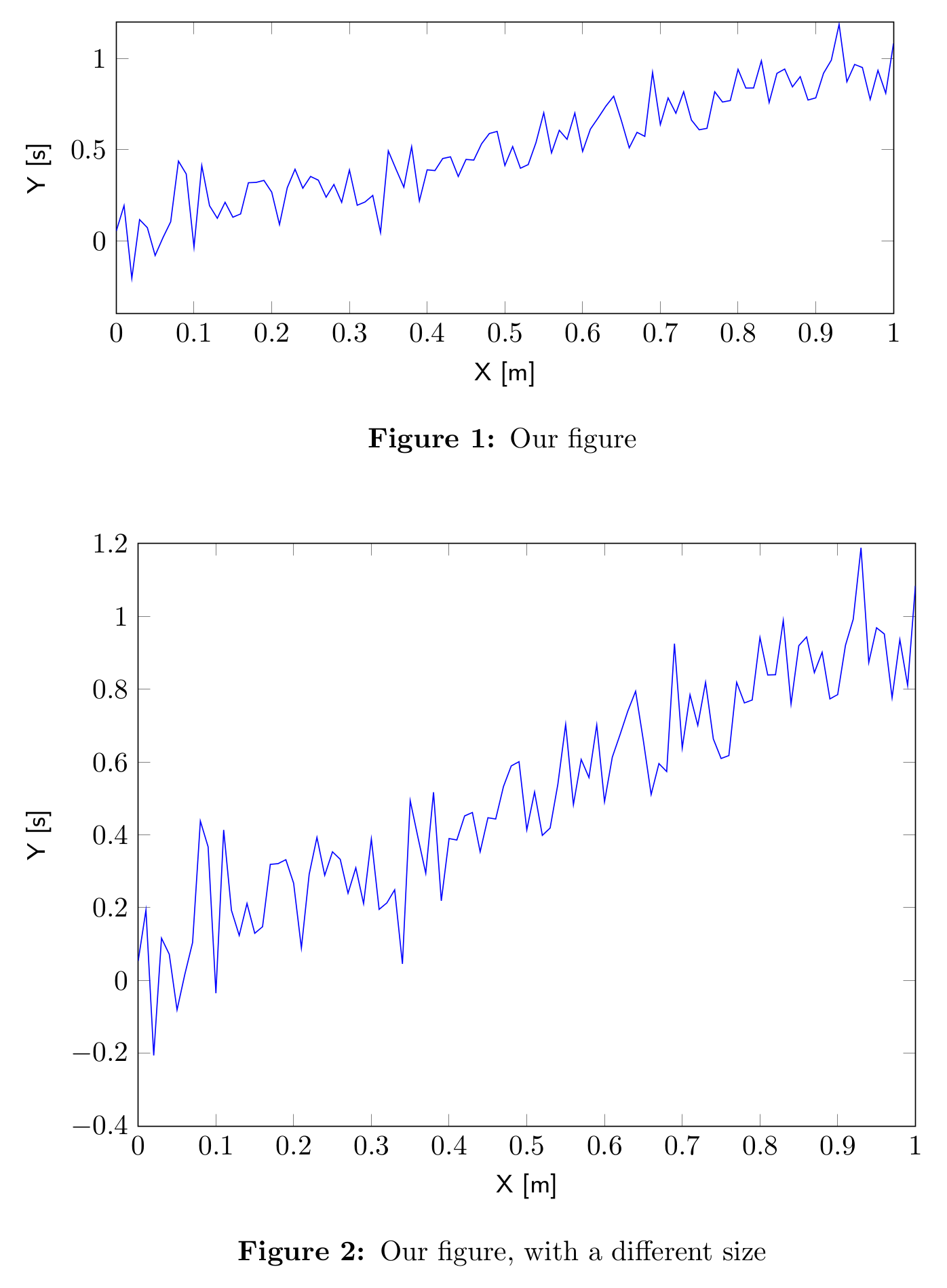
Notice how not only do we have the same figure with two different sizes although we used the same tikz file, but the two figures are both perfectly typeset. Additionally, the lower figure has more ticks on the Y-axis, since its height allows enough space for the additional ticks.